vlaiv

5 hours ago, MilwaukeeLion said:

Helpful thread, ideally I need adjustable barlow or electronic barlow wheel for my set up.  2.5x barlow is close with blue using vlaiv's multiplier  f .76 higher and 229mm fl higher but far off on red f 7.25 high and 2045mm FL high.  With 2x barlow blue is f 8.24 low and 1181mm low but red is f 1.76 low and 645mm high?

 

Honestly, I don't quite understand what you said

But I would like to point something out.

2.4 pixels per Airy disk radius is theoretical optimum sampling value based on ideal seeing and ability to do frequency restoration for those frequencies that are attenuated to 0.01 of their original value. This means good SNR (like 50-100 SNR) to be able to do that, as well as good processing tools that enable one to do it.

In real life scenario, seeing will cause additional attenuation of frequencies (but not cut off like Airy pattern), that is combined with Airy pattern attenuation and cut off. So while ideal sampling will allow one to capture all potential information - it is not guaranteed that all information will be captured. On the other hand, I just had a discussion with Avani in this thread:

where I performed simple experiment on his wonderful image of Jupiter taken at F/22 with ASI290 to show that same amount of detail could be captured with F/11 with this camera. He confirmed that by taking another image at F/11, but said that for his workflow and processing he prefers using F/22 as it gives him material that is easier to work with. So while theoretical value is correct, sometimes people will benefit from lower sampling - if seeing is poor, and sometimes people will benefit from higher sampling simply because post processing and tools better handle such data.

So bottom line to this is that one should not try to achieve theoretical sampling value at all costs. It is still good guideline but everyone should do a bit experimenting (if gear allows for it) to find what they see as best sampling resolution for their conditions - seeing and also tools and processing workflow.

2 hours ago, Pete Presland said:

A very interesting thread @vlaiv thanks for sharing.

Using Dawes limit to solve the resolving power of my C9.25" telescope it can resolve 0.49 arc-seconds.
According to sampling theorem i need to sample at twice the frequency of the signal being sampled. So the ideal resolution for my C9.25" would be to sample at about 0.25 arc-seconds/pixel, which would be no Barlow. Just seems a bit low at F15, let alone F11.2
 

Dawes limit and Rayleigh criterion are based on two point sources separated so that second is located at first minimum of airy pattern. It is usable for visual with relatively closely matched intensity of sources (like double stars). Applying twice sampling to that criterion is really not what Nyquist theorem is about. There are two problems with it:

1. It does not take into account that we are discussing imaging - and we have certain algorithms at our disposal to restore information in blurred image

2. It "operates" in spatial domain. Nyquist theorem is in frequency domain. Point sources transform to rather different frequency representation even without being diffracted to airy disk (one can think of them as being delta functions).

Proper way to address this problem is to look at what airy disk pattern is doing in frequency domain (MTF) and based on that choose optimum sampling.

14 minutes ago, drjolo said:

I have found link to some useful calculators in my bookmarks, and also for CCD sampling http://www.wilmslowastro.com/software/formulae.htm#CCD_Sampling . For green light and 2.9um pixel it gives f/14. 

In some of my "explorations" into this subject, I came with slightly different figure than usually assumed.

Instead of using x3 in given formula, value that should be used according to my research is 2.4

So for camera with 2.9um, optimum resolution for green light would be F/11.2

Here is original thread for reference:

1 minute ago, cuivenion said:

Hi, I'm not going to pretend I completely understood that. But basically you're saying if you choose a gain that is 6db,12db,18db, 24db etc (195, 255, 315, 375) above unity gain then I'll avoid quantization noise?

Yes, unity gain included (it also avoids quantization noise).

1 minute ago, cuivenion said:

Hi, I thought that would be the case, but as I wasn't sure I just played it safe, thanks for the info. The last point has gone over my head a bit. I've not come across quantisation noise. Looks like I've got some reading to do. You've obviously got a deeper understanding of this than me, you couldn't finish off that equation showing the correct gains could you please?

Quantization noise is rather simple to understand, but difficult to model as it does not have any sort of "normal" distribution.

Sensor records integer number of electrons per pixel (quantum nature of light and particles). File format that is used to record image also stores integers. If you have unity Gain - meaning e/ADU of 1 - number of electrons get stored correctly. If on the other case you choose non integer conversion factor you introduce noise that has nothing to do with regular noise sources. Here is an example:

You record 2e. Your conversion factor is set to 1.3. Value that should be written to the file should be 2x1.3 = 2.6 but file supports only integer values (it is not up to file really, but ADC on sensor that produces 12bit integer values with this camera), so it records 3ADU (closest integer value to 2.6, in reality it might round down instead of using "normal" rounding).

But since you have 3 ADU and you used gain of 1.3 what is the actual number of electrons you captured? Is it 2.307692..... (3/1.3) or was it 2e? So just by using non integer gain you introduced 0.3e noise on 2e signal.

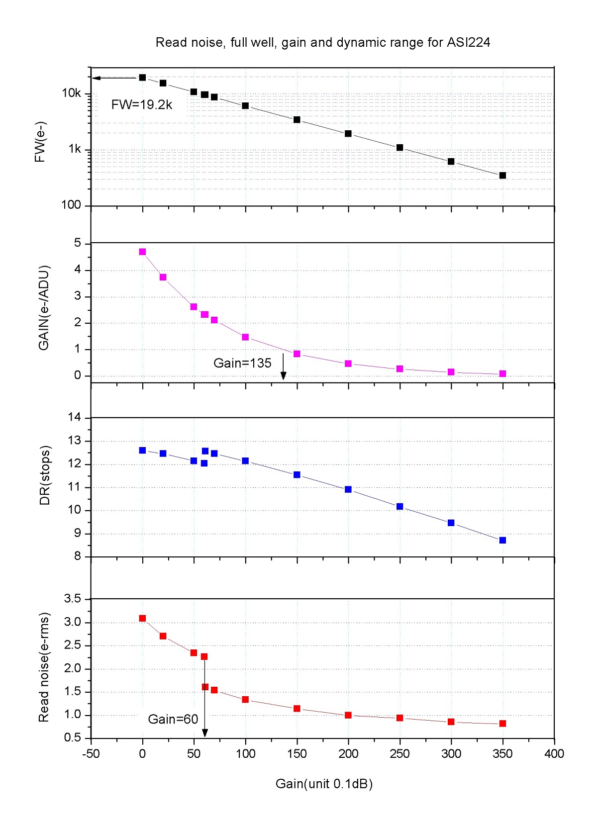
On the matter of gain formula - it is rather simple. ZWO uses DB scale to denote ADU conversion factor, so Gain 135 is 13.5db gain over the least gain setting. So how much is lowest gain setting then?

sqrt(10^1.35) = ~4.73 and here it is on graph:

Ok, so if unity is 135 (or 13.5db or 1.35 Bell), we want gains that are multiples of 2. Why multiples of two? In binary representation there is no loss when using powers of two do multiply / divide (similar to decimal system where multiplying with 10 and dividing with 10 only moves decimal dot) - so guaranteed quantization noise free (for higher gains, for lower gains you still have quantization noise because nothing is written after decimal dot).

DB system is logarithmic system like magnitude. So if you multiply power / amplitude you add in db-s. 6db gain is roughly x2.

(check out https://en.wikipedia.org/wiki/Decibel there is a table of values - look under amplitude column).  Since gain with ZWO is in units of 0.1db - 6db is then +60 gain.

Btw, you should not worry if gain is not strictly multiple of 2 but only close to it, because closer you are to 2 - quantization noise is introduced for higher values (because of rounding) - and with higher values SNR will be higher (because signal is high already).

2 hours ago, cuivenion said:

Thanks, the only problem with the short exposures is I'm losing the star colour because I need to up the gain so there are enough stars for the stacking software to detect. Maybe there's a way to have Pixinsight detect the stars that aren't visible before a stretch, I'll have to look into it. I thought I'd play it safe with this one.

Software should be able to pick up stars regardless of the gain - it is SNR that matters, not if star is visible or not on unstretched image.

You also don't need to go that high in gain, unity should be ok - not much difference in read noise between unity and high gain. But if you want to exploit that last bit of lower read noise, use gain that will give you multiples of 2 of ADU to avoid quantization noise. That would be 135 + n*60 so 135, 195, 255, ...

1 minute ago, cuivenion said:

Having just bought one these I've been reading up a little and I've just come across this. Does this mean you can't calibrate flat frames properly due to this 'internal calibration', as they need bias or dark flats. Is seems that calibration of any sort is going to be tricky if this is happening.

Can be done with flat darks only, no need for bias files.

To be sure - do simple experiment. Take set of flat darks (just basically darks at short exposure - same that you use to get your flats). Then power off everything and disconnect camera. Power on again, use same settings, and do another set of flat darks. Stack each group using simple average stacking to get two "masters". Subtract second master from first and examine the result. Result should have average 0 and have only random noise in it - no pattern present. If this is so, you can simply use following calibration:

master dark = avg(darks)

master flat dark = avg(flat darks)

master flat = avg(flats - master flat dark)

calibrated light = (light - master dark) / master flat

Note that lights and darks need to be taken on same temperature and settings, and flats and flat darks on their own temp, exposure and settings (which ever suit you to get good flat field).

You can on the other hand check if bias is behaving properly by following:

Take two sets of bias subs, and do the same as above for flat darks (two stack, subtract and examine). If you get avg 0 and no pattern - that is good.

Now to be sure if bias work ok, you need to do the following as well.

Take one set of darks of certain exposure (let's say 10s), and take one set of darks with double that exposure (so 20s, same temp, same settings).

Prepare first master as avg(darks from set1) - bias. Prepare second master as avg(darks from set2) - bias. Then create using pixel math following image: master2 - master1*2 and examine it. It should also have avg 0 and no patterns visible. If you get that result then bias functions properly and you can use it (although for standard calibration it will not be necessary as you can use calibration mentioned above).

3 hours ago, mikey2000 said:

I made two master darks with my camera.  One for 120s, one for 300s.  Both at -20C, Gain 0 (The driver calls it 'High Dynamic Range')  (Stretched to view with pixinsight STF)

I would not go with Gain 0 - too much quantization noise. Use Gain 139 preferably or Gain 79 if you want more dynamic range. Scale your exposure length so you don't get too much saturation. Even if you saturate bright stars, there is a way around it - just shoot some short exposures to recover signal in brightest areas.

2 hours ago, wimvb said:

No, just that temperature increases during an exposure, such that amp glow is worse (more than linear) at longer exposure times. You may have noticed that images with sub frame exposures in excess of about 600 s are very rare. Not only are they not needed because of the low read noise, but they are actively avoided because of the increased amp glow. Even if amp glow can be removed by careful calibration, the random shot noise that is associated with it can not.

How long it takes for the increased temperature to reach a stable level, I don't know, but it is probably several tens of seconds.

I don't think that dark current shot noise is really a problem. Look at this graph for ASI1600

At -20C dark current is 3.72e at 10 minute exposure, so associated shot noise would be 1.92e or order of read noise. That is low dark current noise in 10 minute sub.

From the graph we can see that doubling temperature is around 7C for temperatures bigger than 0C, and even a bit bigger for lower temperatures. So even if amp glow is +7C warmer (and I would be surprised that there is such temp differential across the surface of the chip without causing mayhem), dark current in amp glow area will still be less than x2 dark current elsewhere and associated noise would be less than x1.41 - again on 10 minute sub, not something to worry too much about. For amp glow area to be x4 higher in dark current - thus having x2 more noise than elsewhere, that part of sensor would need to be almost 15C hotter than the rest!

If peak temperature in amp glow area is not dependent on surrounding temperature, but on set point cooling only, then it calibration should work each time, but yes one would have to prepare master dark for each exposure length.

1 hour ago, wimvb said:

Btw, the imx183 image you posted, looks more like radiation than amp glow. Very strange. Could this just be a faulty sensor? Or a light leak maybe.

I've seen it before, it looks like it is very common on Sony CMOS sensors. My ASI178MCC has amp glow that is cross between ASI1600 and that one on the image. Corners are affected like in ASI1600, but in each corner there is "source of rays".

Here is what it looks like:

And to my knowledge, my ASI178MCC calibrates ok regardless of strange amp glow.

1 hour ago, wimvb said:

On ASI cameras, amp glow is generated by circuitry on the sensor, and this can't be shut off during exposure or read out. That's why ZWO have such a hard time trying to reduce it. The Peltier cools the whole sensor, but there are still variations across the sensor, hence amp glow.

Ok, still not following (sorry about that). Well I do understand what you mean I just don't understand fully consequences of that.

So you are saying, there are parts of the chip that are at different temperature than the rest of the chip? Right?

Do you have any idea how that temperature behaves in time?

1. It is just a patch of sensor surface where temperature is higher then the rest of the chip but stable - let's say sensor is mostly at -20C but corners are at -18C

2. When there is no exposure going on, whole sensor is at -20C and when exposure starts, sensor remains at -20C but selected few patches in corners start rising in temperature

2a) they rise asymptotically to a certain value quickly (like in few seconds)

2b) they rise asymptotically to a certain value slowly (thus not really reaching that value in common exposure times)

7 minutes ago, wimvb said:

Yes, the casing will be warmer, but the whole idea of Peltier is to keep a fixed temperature on the sensor. Your argument doesn't take Peltier power into account. With a higher ambient temperature, the heat flow will be larger.

Not sure how is that related to amp glow if we assume it is due to build up of heat on adjacent component and it is being fed into sensor via metallic circuitry. Sensor is kept at constant temperature because all excess heat is taken away by Peltier. If amp glow is rising faster than dark current - that means that part of chip is at higher temperature than the rest of the chip, and it is accumulating heat (if it were only at higher temperature but stable we would not be in trouble, since there is time linearity at different temperatures). Some of that heat will indeed be taken away by Peltier via sensor, but if it is rising, it will also be in dynamic with its surroundings - some of the heat will dissipate elsewhere because not all of it is being drawn away by Peltier. Otherwise amp glow temperature would also be stable. And if it is dissipating heat by other means than Peltier - speed of dissipation will depend on temperature gradient between that component and wherever that heat goes to.

1 minute ago, wimvb said:

With an active cooling element (peltier) rather than passive, fan cooling, ambient temperature should be less of an issue. Once the temperature us set, ambient temperature only determines how hard the cooling system has to work. The only times I've had problems with this was when shooting darks. I have my camera in a black box (no pun intended), and the temperature rises a few degrees during capture. If the set point is close to what the camera can handle, the set temperature may not be reached. But as long as the set temperature is welk witjin the camera's limit, I've never had a problem.

Btw, I suspect the ASI's temperature sensor to be a bit on the optimistic side.

Regardless of peltier cooling, if amp glow is produced by heat buildup - this means there is excess heat that is not being removed via peltier cooling. Such heat will be dissipated by regular means of heat transfer to surroundings (conduction and convection). Efficiency of such heat removal will depend on environmental temperature. Even if we look at camera as closed system, camera casing will be at different temperature (it is used to remove the heat from the system) depending on actual surrounding temperature. In cold environment casing will remain relatively cold. In hot environment casing will become hotter and hence everything inside casing will be at higher temperature, meaning less effective heat dissipation of amp glow producing component - bigger thermal build up in it - stronger amp glow.

I guess temperature sensor does not need to be accurately calibrated as long as it is "reproducible". Whether I'm shooting at -18C while it says -20C, I don't think it matters as long as each time I tell it to go to -20C it remains on -18C

On topic of CMOS amp glow:

https://www.cloudynights.com/topic/599475-sony-imx183-mono-test-thread-asi-qhy-etc/page-3

There is some interesting discussion and data.

One thing that intrigues me is ray like feature in amp glow in CMOS sensors. That is not something I would expect from heat. It looks more like there is some sort of electron build up due to electric / magnetic fields from adjacent circuitry rather than heat. Due to fast readout there are components in CMOS sensors that operate in Mhz range. Could this all be due to rouge EM radiation?

2 hours ago, wimvb said:

Here is where theory goes awry. Amp glow does not scale linearly with time. Amp glow is due to an uneven heating of the sensor. A local increase in temperature leads to a local increase in dark current. If the local temperature were constant, amp glow would increase linearly with time. But temperature increases with time, probably until a steady state is reached, and amp glow will increase more than linearly with time. This is the reason why amp glow in ASI cameras can't be calibrated out completely with darks taken with a different exposure time.

Very good point, I have not look into it but it looks like I'm going to have to.

There is another explanation why ASI1600 would not be able to calibrate properly with different exposure darks. It turns out there is sort of "floating" bias with ASI1600. Whether this is something implemented in drivers or it is feature of sensor itself, I have no idea, but it turns out that bias level drops with exposure length. I've seen while measuring sensor data that average levels for 1m exposure are lower than that of straight bias for same settings and temperature. I was under the impression that it stabilizes at some point, but it might not be so. Only thing that I've noticed is that after 30s or so average value starts rising - as one would expect due to buildup of dark current.

If sensor indeed changes bias level depending on exposure length (and it seems so) it would also be a reason why different exposure darks would fail at calibration. One needs bias removed prior to adjusting dark current levels.

On the amp glow topic - it sounds reasonable what you are saying but that would have another implication. There would be difference in amp glow between darks of same exposure and settings taken under different surrounding temperature conditions. Equilibrium in amp glow would depend on efficiency of heat dissipation from the system - which is higher in cold environment than it is in hot. I would expect amp glow to be less in darks taken on a cold night outside vs darks taken at room temperature. I'm shooting my darks indoors, and calibrate with them lights taken in at least 10C colder conditions. I've not noticed residual amp glow after calibration. I'm not saying that it is not there, I just have not seen it, and it might well be because I was not paying attention.

If it turns out that there is indeed dependence of amp glow to ambient on same temp and settings, I guess one would need to have couple of sets of master darks taken at different ambient temperatures (like summer darks and winter darks and one set for spring / autumn or something like that).

I don't really know the nature of amp glow in CMOS sensors. With CCD sensors it was indeed amp glow - since CCDs have single amp unit, and if that electronics was too close to sensor it would cause problems - heat travels via circuitry back towards the CCD (metal conducts electrons one way but equally good heat in opposite direction). With CMOS sensors there is amp unit associated with each pixel, so I doubt what we see and call amp glow is indeed related to amp unit(s) with CMOS.

3 hours ago, mikey2000 said:

Thanks for the tips everyone.  Vilav - is your procedure meant for CCD sensors?  I have a CMOS.

I think Olly may have hit the nail on the head - Experiment and see what happens. 

 

I think I was just being lazy - someone else must have done this before me, with this camera!

It is meant for both CCD and CMOS sensors, well, at least "well behaved" ones. It is proper calibration method in sense that it removes all but light signal from light frame and correctly applies flats (only on light signal).

I have ASI1600 myself and that is what I use for calibration.

On a side note, well behaved sensor is one that:

- has predictable bias signal (read noise is random but bias signal is always same for every pixel)

- has dark signal dependent on temperature and exposure duration (linearly grows with exposure length on fixed temperature). Can have uneven dark current (amp glow), but it needs to behave as said per pixel

- has linear response to light.

Yes you can skip bias frames, not only that you can skip them, they are not needed with set point cooled cameras, if you use darks of matching length and temperature.

Calibrate like this:

master dark = avg(darks)

master flat dark = avg(flat darks)

master flat = avg (flat - master flat dark) or
master flat = avg(flat) - master flat dark

calibrated light = (light - master dark) / master flat

Use as much calibration frames as you can. Use at least 32bit precision, and that is it.

18 hours ago, MartinFransson said:

Thanks for the analysis! Two questions then, considering the problem is two fold:

1. Why would the distance be anything but spot on since I am using the recommended gear for this. The ZWO lens adapter is specifically adjusted to get the right distance.

2. What could cause the tilt? Sensor not mounted properly? Everything else is just put together and the lens itself has a flat plane.

 

Do you have exact matching lens adapter for ASI1600? Not all ZWO cameras have same T2/2" thread - sensor distance, so lens adapter should be adjustable for flange distance (which for Canon EF / EF-S is 44 mm).

If adapter is adjustable is it lockable (like with screws?) it can cause tilt if not tightened properly, well, anything can cause tilt if not tightened properly (and sometimes even if tightened properly but manufactured to wrong specs).

This looks familiar, I used to get star shapes looking like that, and problem is two fold.

First is sensor / lens distance - you need to get it spot on for flat field. What you see in image above is mostly astigmatism. Right side of the image is in focus but has astigmatism - cross shape, while left has out of focus astigmatism - elliptical shape - bad sensor / lens distance.

Second is that you have some sort of tilt in optical train - sensor is tilted in relation to focal plane. Right side in focus, left a bit out of focus.

Ha subs still display this sort of behavior but it is much less pronounced because star shapes in corners when using refractive optics depend on wavelength of light. So in this particular configuration Ha (red part of spectrum) is less affected, but green would be a bit more, and blue still more than that.

1 minute ago, GalileoCanon said:

So vlaiv at 1070 pixels, the moon will (roughly) fill 1/2 of my image vertically and 1/3 of my image horizontally? That really clears things up in extreme detail. Thanks!!

Yes, well, probably closer would be to say 1/4 horizontally (3888 is close to 4000) and 1/2.5 vertically. But do have a look at Stu's post from above to get the feel of the size of moon on image - it clearly shows how much of image would Moon take up.

So you are interested in two things (if I'm getting that right):

1. how larger object would be compared to certain lens?

Simple ratio of focal lengths of a given lens to 700mm of your reflector (provided we are talking about same camera used).

2. what would actual size of object be on your image?

For this you need to know angular size of the object and pixel size of your camera (that is roughly sensor size divided with resolution, so in your case it would be 5.7um - or 5.7 micrometers, or you can look it up online).

Then you need to use following formula:

http://www.wilmslowastro.com/software/formulae.htm#ARCSEC_PIXEL

To get resolution of image in arc seconds per pixel - in your case it is 1.68"/pixel

Use that value, and divide target size (in arc seconds) and you will get number of pixels that target will be on image. So for Moon which is 30 arc minutes (that gives 1800 arc seconds) will be ~1070 pixels wide on the image.

In all seriousness, telescope without eyepiece or camera is projection device rather than magnifying device. As pointed out by ronin, telescope forms image of object on focal plane of a certain size. That size depends on focal length of telescope and actual size and distance of object (or in other words - angular size of object).

Magnification would imply conversion of scale of single unit - so we can say that Moon is magnified x60 if angular size of Moon is 30 degrees given that we see Moon without magnification to be 30' (or 0.5 degrees). Telescope on its own does not convert scale of single unit - it does unit conversion (projection) - from angular to planar / spatial so we end up going from angular size to length.

Now eyepiece / telescope combination does magnification. Telescope / prime focus camera does not do magnification in that sense, it is also projection device - with addition of sampling rate. Sampling can be seen as number of pixels per mm or number of pixels per angular size - this is what gives illusion of "magnification" or zoom to an image. It is not really magnification or zoom, it is just sampling resolution. Same image can be both small or big, depending on monitor that we use to display it, and distance to observer - look at any image on computer screen from "normal" distance and then move 10 feet away - it will look much smaller   (but it is the same image, sampled at the same resolution). So resolution is not measure of magnification / zoom in normal sense.

1 hour ago, ronin said:

No magnification, you need an eyepiece and an eyeball for magnifiv=cation.

What youy get is an image size, defined by the tangent of the angle subtended by the object multiplied by the scope focal length.

If you put a 2x barlow in then the object size is doubled.

So moon = 0.5 degrees, scope appears to be 700mm so the image is:

S = tan(0.5)*700 = 6.1mm.

So as you see, telescope is not magnifying at all!

It is minifying - making Moon that is 3474 km in diameter, appear to be only 6.1mm!

7 hours ago, Merlin66 said:

Vlaiv,

Glad you found that error....

I think you need to revisit Suiter's "Star Testing Astronomical Telescopes". On p61 he models a simplistic analysis of the Airy Disk based on the Heisenberg uncertainty principle and comes up with an answer close to the 1.22lambda/D.

I have yet to see an astronomical image showing the Airy Disk. (On the bench a pinhole optical system is usually used to generate the Airy disk images normal see in the text.) It needs at least a >f30 system and absolutely perfect conditions. Suiter's work is based on VISUAL and high magnifications.

What we record is the PSF of the seeing disk.

Re Sampling (See Suiter, p41) and the MTF Chapter 3.4. Eversberg and Vollmann in their "Spectroscopic Instrumentation" p 76 discuss at some length the issues of effective sampling - starting with the Nyquist criterion - they advocate at least a sampling rate of >3. (This again is based on the PSF rather than the "absolute" Airy Disk)

I'd also refer you to Schroeder's "Astronomical Optics". 

 

Hm, I did similar analysis recently - Heisenberg vs Huygens–Fresnel principle and it turned out that there is numerical mismatch, but I did not look at Suiter's example, will have a look.

As far as I understand, circular aperture in telescopes (obstructed or clear) produces Airy pattern as PSF on focal plane for point source aligned with optical axes. If we explain the phenomena in classical terms (Huygens-Fresnel) - it is because on aperture plain there are infinite number of points acting as point sources for spherical waves (all in phase, because incoming wave front hits them in phase) and interference of those waves at focal plane gives raise to Airy pattern.

On the topic of Airy PSF vs Seeing PSF

- we are indeed applying wavelets on stacked image that has been under influence of seeing, but actual final image, due to lucky imaging has 2 blur components - Airy PSF and Gaussian distribution of Seeing influence. Each stacked frame was blurred by particular seeing PSF and each frame had different seeing PSF applied to it, but we align and stack such frames which leads to central theorem - sum of individual random seeing PSFs will tend to have Gaussian shape. Each frame has Airy PSF of telescope applied to it, but that is each time the same.

Now property of Gaussian PSF is that it attenuates high frequencies but there is no cut off point - all frequencies are present, and therefore can be restored with frequency restoration - power spectrum of Gaussian PSF is Gaussian (fft of gaussian is gaussian). So cut off that is applied is still Airy PSF cut off, and all the seeing attenuated frequencies can be restored given enough frames.

On the matter of sampling and Nyquist criterion in 2d - it is simple, on square grid you need x2 sampling rate (on rectangular grid you need x2 sampling rate in x and x2 sampling rate in y but if we use square grid units are same in x and y) to record any planar wave component. Imagine sine wave in x direction (y component is constant) - it is the same as 1d case so we need x2 sampling rate to record it. Also imagine sine wave in y direction (x is constant) we need x2 sampling rate in y direction to record it - same as 1d case. Now for any sine wave in arbitrary direction - projection on x and y axes will have longer wave length - so it will be properly sampled with x2 because each component will have lower frequency than when wave is in x and y direction.

So 2d Nyquist is clearly same as 1d, on square grid we need 2 samples per shortest wavelength we want to record.

Now, I did not do my analysis mathematically, but I will present what I've done and how I came to the conclusion, which I believe is supported by above example.

I generated Airy PSF from aperture, both clear and obstructed (25%) and made Airy PSF be 100 units (pixels in this case) in diameter. Here is screen shot of clear aperture PSF (normal image, stretched image to show diffraction rings, profile plot, and log profile plot to compare to Airy profile):

This is how obstructed aperture looks like (same things shown in same order):

you can clearly see energy going into first diffraction ring - cause of lower contrast when doing visual.

Now lets examine what MTF graph looks like for both cases:

First clear aperture:

And obstructed

If you compare those with the graph in the first post - you will see that they match.

Now question is, at what frequency / wavelength does cut off occur? We started with airy PSF with disk diameter of 100 units. Now I did not do calculation but I rather "measured" place where there is cut off. On this image log scale is used, so where central bright spot finishes that is cut off point:

"Measurement" tells us that cut off point is roughly at 40.93 pixels per cycle. This means that we need our sampling to be 40.93 / 2 units or ~20.465 units long.

How big is that in terms of airy diameter? Well airy diameter is 100 units, so let's divide those two to see what we get: ~4.886

So in this case we get factor of ~ x2.45 of airy disk size for proper sampling resolution.

When I did my original post I also did measurement and found that rounded off multiplier is x4.8 in relation to diameter, or x2.4. So true value is somewhere in that range x2.4 - x2.45. We would probably need rigorous mathematical analysis to find exact value, but I guess x2.4 is good enough as a guide value - most people will probably deviate from it slightly because there is only limited number of barlows out there

So to recap:

going x2 Airy disk radius - undersampling (you might miss out on some detail, but really not much - it is 4pp example from first post)

going x2.4 Airy disk radius - seems to be proper sampling resolution for planetary lucky imaging (if you buy into all of this )

going x3 or x3.3 - you will be oversampling, thus loosing SNR with no addition detail gain (it is 6pp image from first post)

Ooops

I just realized something. x2, x3 and x3.3 sampling was given in relation to airy disk radius, not diameter.

My example was talking about x4.8 of airy disk diameter. This means that actual value comparable with those listed is x2.4 of airy disk radius. So yes, please if you feel confident in my analysis (and I'll post some more info to back up all of this tomorrow, now it's getting a bit late), use that resolution - it will provide you with better conditions for planetary imaging than other "optimal resolutions" quoted. It will provide more detail than x2 and it will have higher SNR per frame than x3 and x3.3 (but same amount of detail - max possible for given aperture as those).

Yes, that would pretty much be it.

You take size of airy disk for blue (highest frequency, shortest wavelength) and find the size of Airy disk in seconds of arc (formula is 1.22 * lambda / aperture diameter - this one is for angle to first minima in radians so you need to multiply by 2 and convert to arc seconds, both lambda and aperture are in meters). Once you found your airy disk diameter, divide with 4.8 - that should give you resolution that you should be sampling at and from that you calculate FL.

So for first scope you mentioned:

2 * 1.22 * 0.000000450 / 0.3  radians = ~ 0.755" diameter of airy disk in blue (450 nm)

this should give you resolution of ~ 0.1573"/pixel.

For camera with 3.75um, FL required for this resolution would be: 4940mm, so you are looking at x3.25 barlow. You will not miss much by using x3 barlow (don't need to sample blue to max, you can go with green instead, blue will be undersampled a bit but it will not make too much difference).

Now, this is all theoretical more than practical - that is maximum achievable resolution with perfect optics, perfect seeing and frequency reconstruction (with wavelets or something else).

As such this should be guide to max usable resolution above which there is simply no point in going higher. In real use case scenario you might not even want to go with such high resolution - it requires exceptional seeing, and with increase of sampling resolution - SNR per frame will go down - so you need plenty of good frames for stack in order to recover SNR to acceptable levels to be useful for frequency reconstruction.

I did all of this analysis because I was always intrigued by the fact that there are many different "optimal" resolutions out there in the "wild", and I wondered which one is correct. Now, x2 airy disk is somewhat related to visual - that is how x50 per inch or x2 in mm for max useful magnification is derived. That and average human eye resolution of 1 minute of arc. But eye can't do what computers do with frequency reconstruction - we can't make our eye amplify certain frequencies - it sees what it sees. This is the main reason behind x3 and x3.3, I guess people just realized that sampling on higher resolution does indeed bring more detail after wavelets (and certain article that does similar analysis as above, but for some unknown reason quotes x3 for 2d Nyquist, and gives wrong interpretation of cutoff wavelength that rises from given airy PSF).

Central obstruction absolutely plays no part for imaging. If you look at MTF graph, central obstruction has same cut of frequency, and only impact is to attenuate a bit more certain spatial frequencies (larger details will have a bit less contrast compared to unobstructed scope - this is important for visual, and you often hear that refractors, having no CO, have better contrast on planets - that is the reason). With frequency reconstruction this is of no importance.

There are a few recommendations around the web regarding the optimum planetary resolution with respect to aperture of telescope.

I've found values x2, x3 and x3.3 pixels per airy disk.

While playing with ImageJ and generation of different airy disk patterns (obstructed, clear aperture, different sizes) and examining results, I've come to following conclusion:

Optimum resolution for planetary imaging, when including wavelet post processing is x4.8 pixels per airy disk

My conclusion is based on following: x2 sampling (as per Nyquist 2d sampling in rectangular grid) of frequency that is attenuated to effectively 0 if one examines perfect airy disk pattern.

If we look at the following graph representing attenuation depending on frequency (well known MTF graph - which represents 1d cross section of power spectrum of airy disk pattern, for clear and obstructed aperture)

(dashed line - clear aperture, solid line obstructed aperture)

we can see that for attenuation of 99% we are approaching cut of frequency at almost 99%, this means that frequency very close to cut of frequency will be at 1% of strength of original. For visual observation that is significant because loss of contrast is great at those frequencies, but when one applies frequency restoration and enhancement (effectively boosting contrast) of wavelet algorithm - we can see that this frequency can easily be restored by multiplication with factor of 100 (something eye can't do, but computer can easily with appropriate algorithm).

Now in my simulation of airy disk influence, I've found that for 200mm aperture with 25% central obstruction, cut off wavelength is ~0.5333" - meaning optimum sampling rate would be ~0.2666"/pixel or in relation to airy disk size of ~1.28" (510nm light) that equals x4.8 airy disk diameter.

In order to demonstrate these effects I've made "virtual recording" of Jupiter (original high resolution image used: http://planetary.s3.amazonaws.com/assets/images/5-jupiter/20120906_jupiter_vgr1_global_caption.png)

sampled at x3pp, x4pp, x4.8pp, x5pp, x6pp (in relation to airy diameter) of high resolution image convoluted with airy disk psf. So images represent perfect 25% obstructed optical system without seeing influence.

This is reference image (no convolution, sampled at 6pp):

And this is result of convolution without frequency restoration (sampled at 6pp):

Next I did different sampling resolutions, applied wavelets to each, and rescaled for comparison (scaling was done with bicubic interpolation), so here is result 6pp, 5pp, 4.8pp, 4pp and 3pp in that order from left to right:

It can be seen that first 3 images look almost identical, while x4pp starts to show little softening and x3pp (as usually recommended for planetary) shows distinct lack of detail compared to others.

I also made a zoom of section around GRS - this zoom was made using nearest neighbor scaling (so individual pixels can be seen) - to evaluate small scale differences:

In image with x4pp contrast starts to suffer and x3pp lacks both features and contrast, while first 3 (6, 5, 4.8pp) show virtually no difference.

So, there ya go, it looks like x4.8 is the way to go with planetary imaging